Georeferencing & digitising
Much valuable geospatial data remains in analogue format, e.g. printed maps or lists of coordinates. This session will cover the processes of georeferencing (assigning explicit geographic coordinates to scanned images) and digitising (creating vector geospatial layers from images and other reference material).
Prerequisites
- Georeferencing a scanned map (Video, Martin Hinz)
- Digitising objects from georeferenced maps (Video, Martin Hinz)
Practical
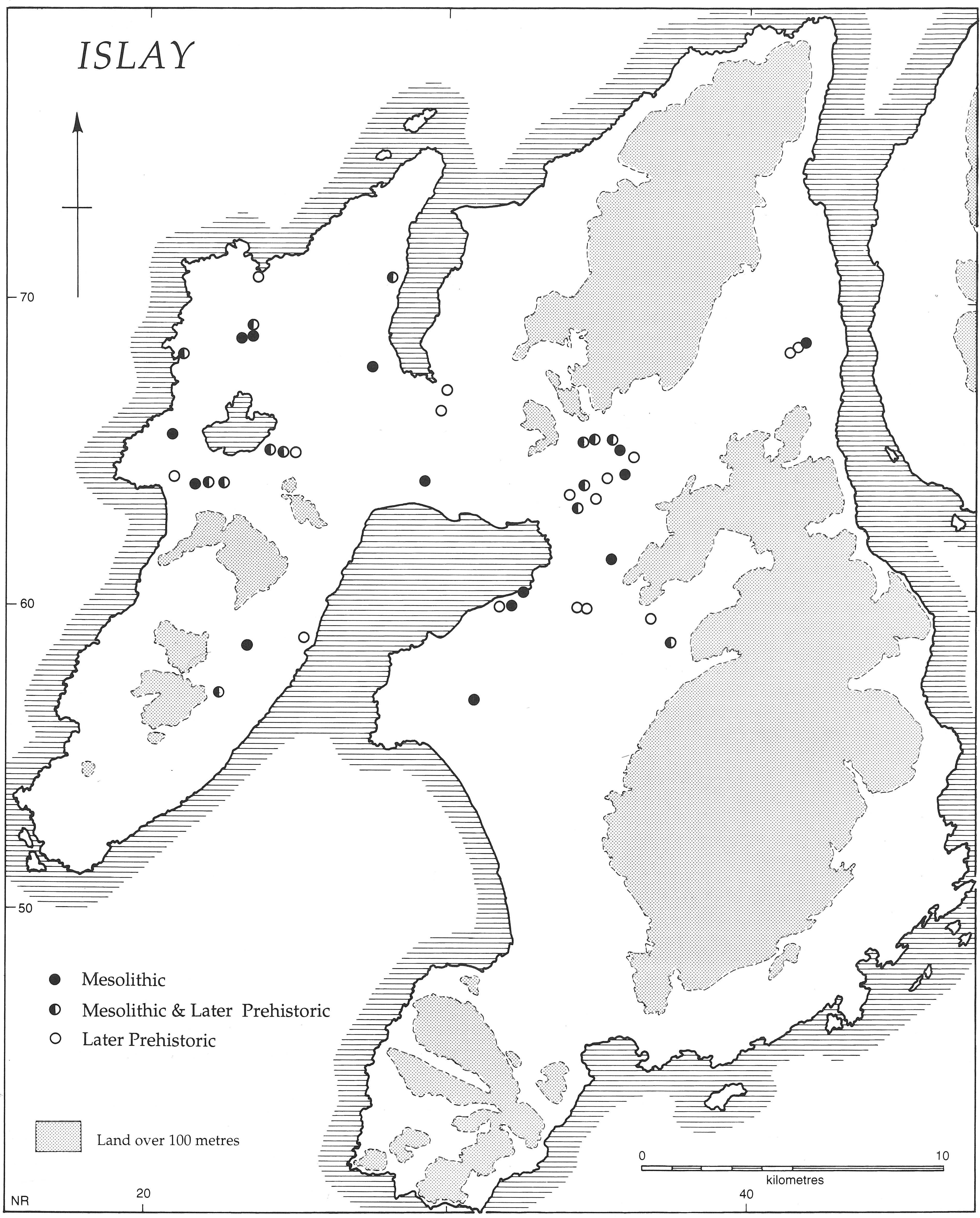
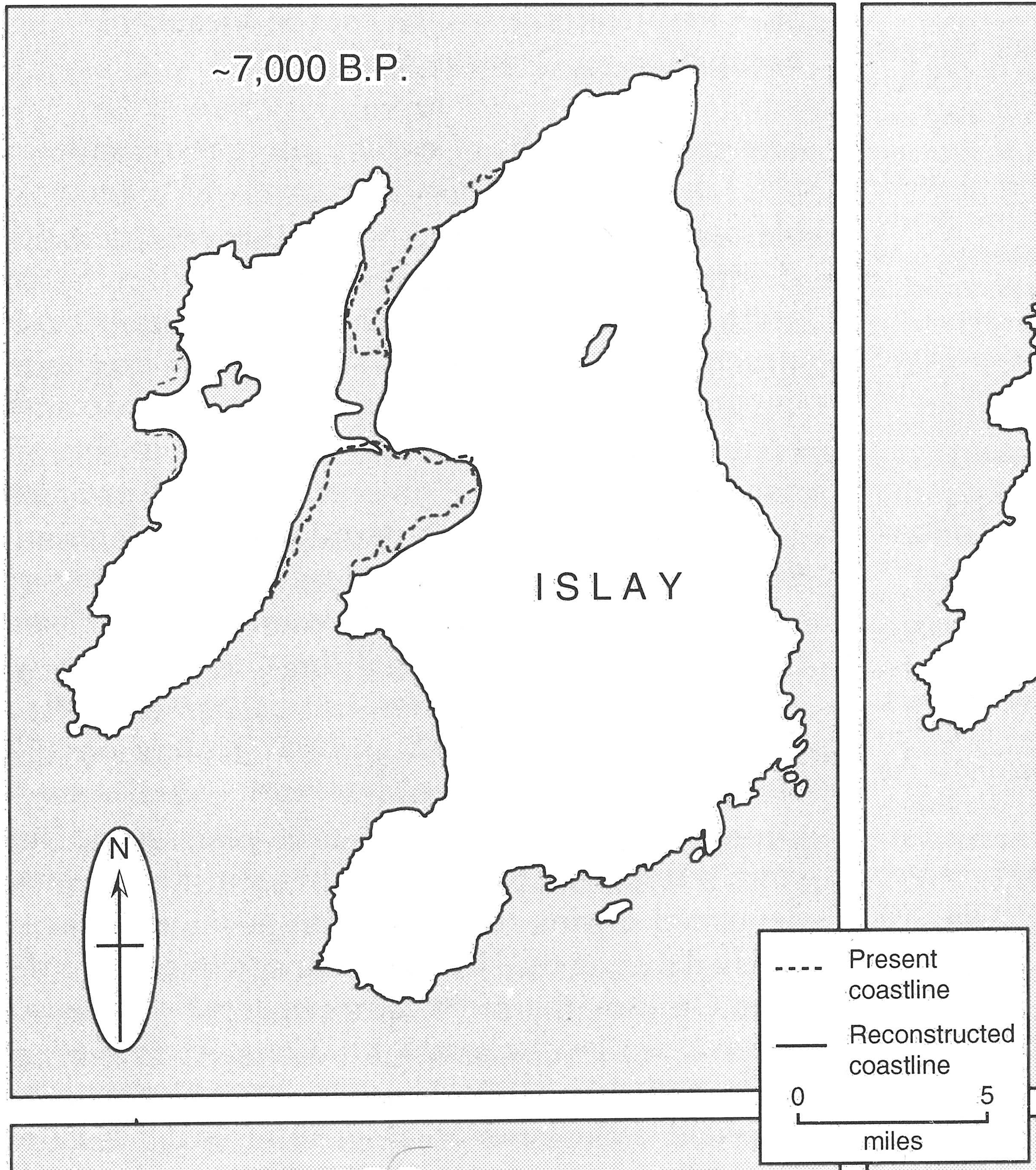
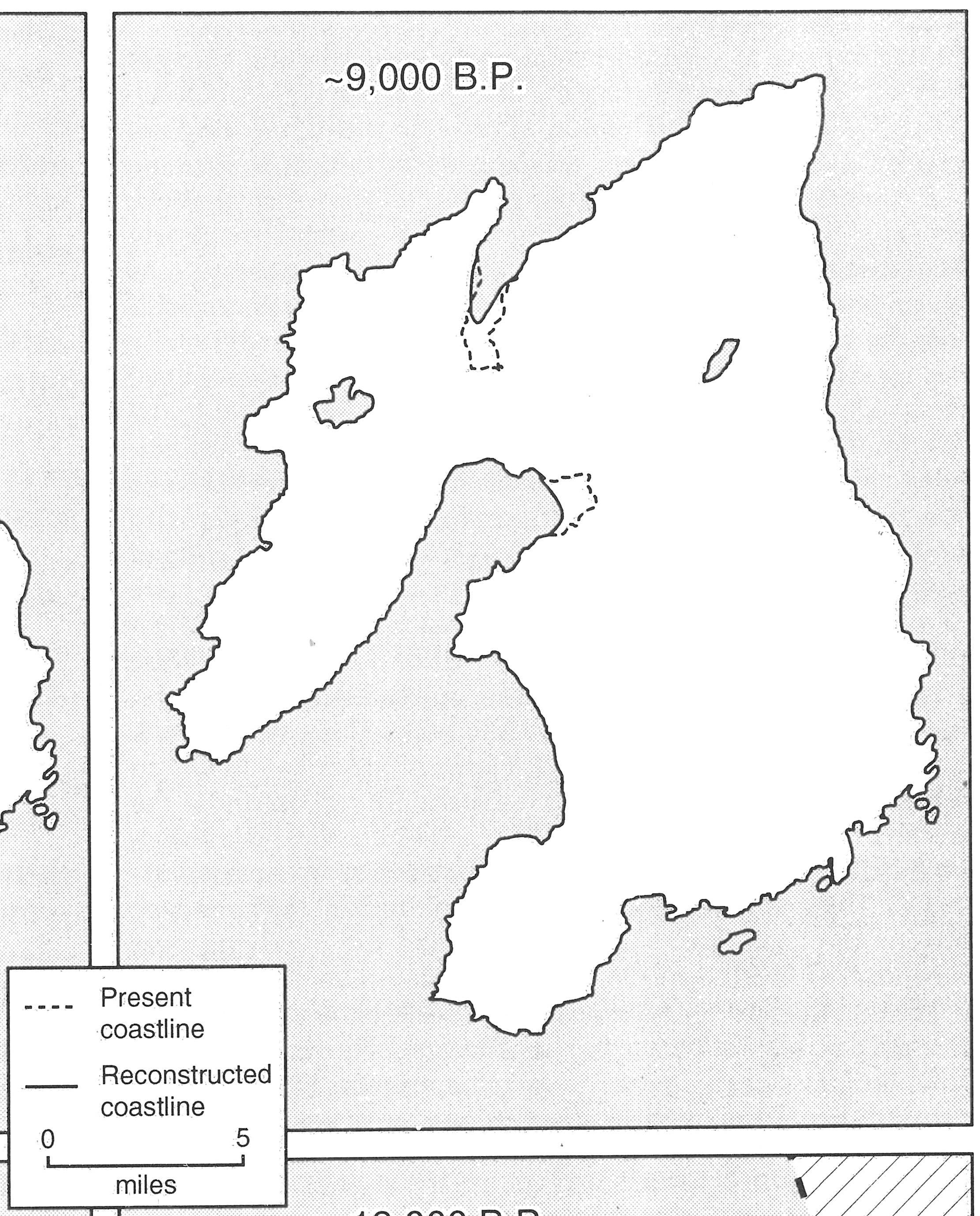
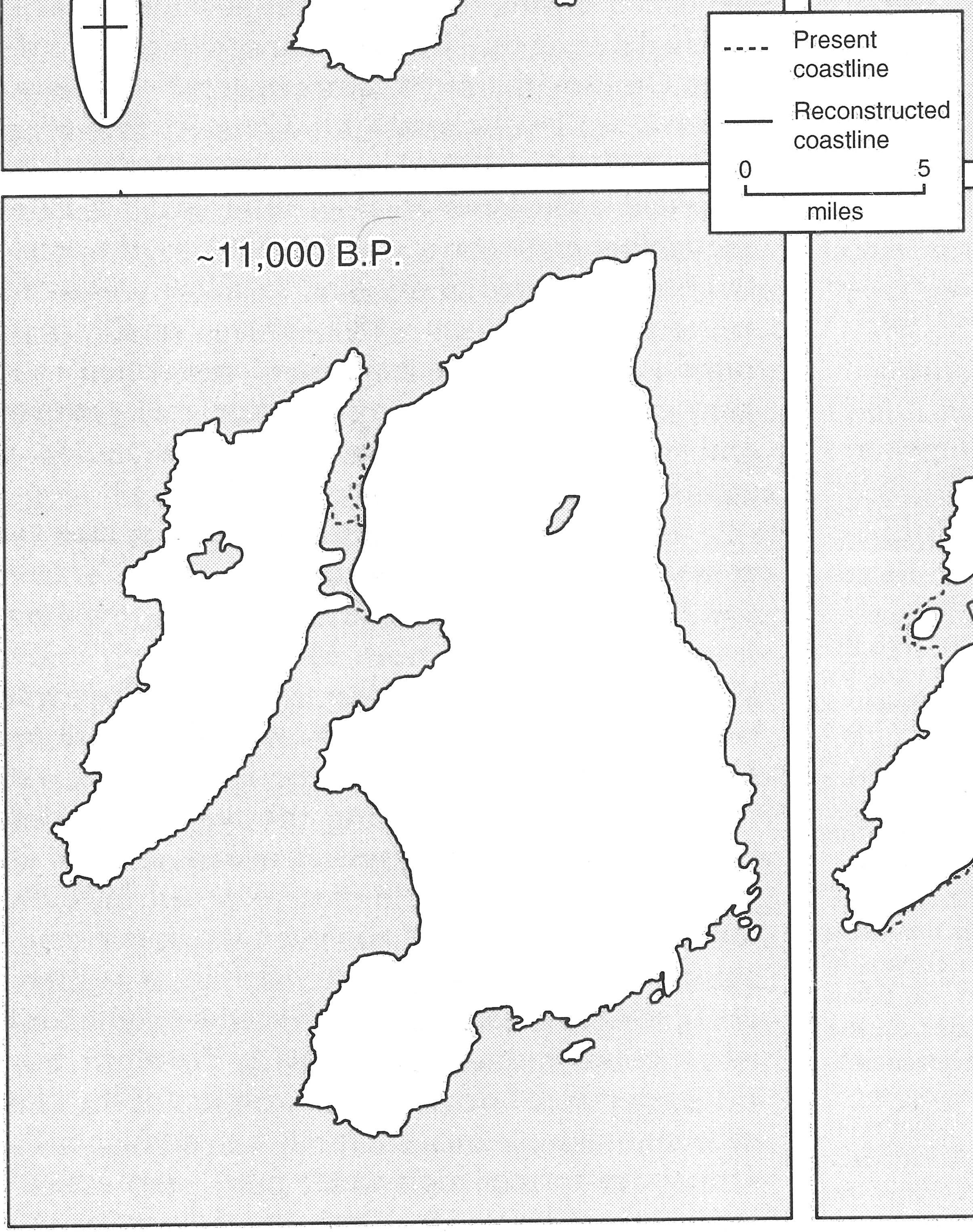
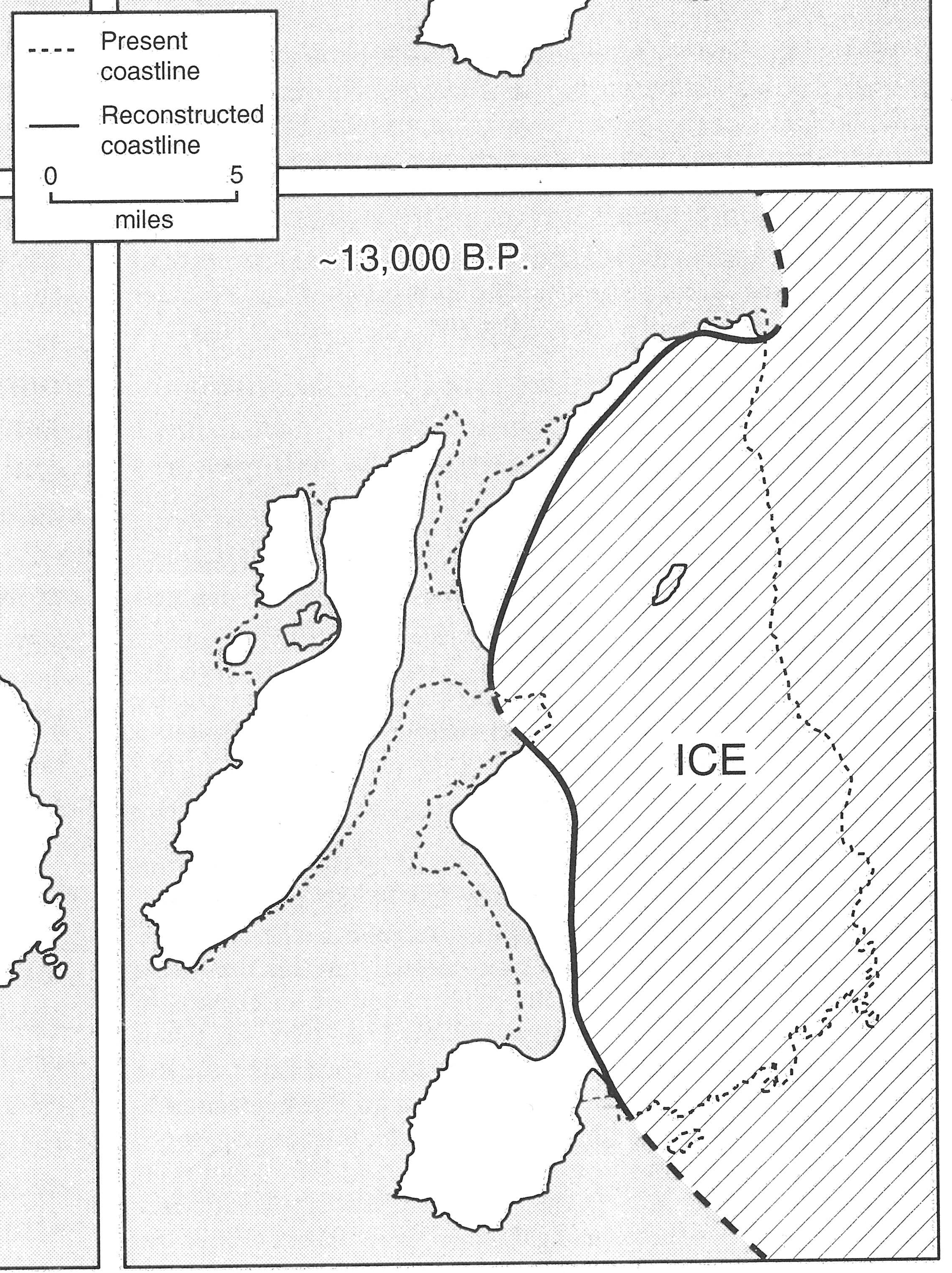
We will georeference and digitise two datasets from Islay that will be useful in our later modelling work: the location of sites, and a reconstruction of the past coastline.
Data
- islay_sites.jpg – map of Mesolithic and later prehistoric sites on Islay (Mithen et al. 2000, fig. 4.2.15)
- Maps of reconstructed past coastlines of Islay (Mithen et al. 2000, fig. 3.4.14):
Georeferencing
Georeferencing is the process of assigning a coordinate reference system (CRS) and geographic coordinates to an image that does not have them, e.g. a scanned paper map. It involves two stages: first defining control points (points on the map with known locations) and then defining the transformation used to fit the source map to the desired coordinate reference system. There are in turn two basic ways to define control points: by using known coordinates (e.g. from a grid, landmark, or cross-referencing with a table) or by matching features with another, already digitised, map of the same area. We will try both in this practical.
- Add the map images to your Islay project and open it in QGIS.
- Change the Project CRS to
OSGB36 / British National Grid(EPSG:27700)- This is the projection used in the two Islay maps.
- Open the Georeferencer (
Layer → Georeferencer) - Use the
Open Raster...button to add islay_sites.jpg to the Georeferencer.
Luckily, this map has some grid references included in the frame of the map. These reference the British National Grid and are in the format NRXXYY, where ‘NR’ is a map sheet and XX and YY are the easting and northing coordinates in kilometres. We can look up the geographic coordinates of the corners of these grid squares, for example at https://britishnationalgrid.uk/. It’s not explicitly stated, but let’s assume that the origin (lower left corner) of the map is at grid reference NR1540.
- In a browser, open https://britishnationalgrid.uk/ and navigate to Islay
- Under ‘grid reference’, change ‘six-figure’ to ‘four-figure’.
- Back in the Georeferencer, select the
Add Pointtool and click on one of the corners of the grid squares. Then input its X and Y coordinates.- Refer back to the website from steps 5–6 to find these coordinates.
- Repeat step 7 until you have at least three control points.
- Q: What is the advantage of picking more than three points?
- Open the
Transformation Settingswindow and tick ‘create world file only’- This means the image will not be ‘warped’, just have coordinates attached to it. We can do this because the source and target CRSes are the same (British National Grid).
- Click
Start Georeferencing. If all goes well, you should now see a georeferenced version of the map in the main QGIS window.
Now we will georeference the maps of the Islay coastline. Unfortunately these don’t have grid references, but since they’re of the same place, we can piggy-back off the work we’ve already done.
- As before, load one of the coastline maps into the Georeferencer.
- When asked, you do not need to save the control points from the previous steps.
- Pick a place on the coastline and add a control point, but this time, instead of entering coordinates, click the
From Map Canvasbutton and click on the corresponding point on the map you have just georeferenced. - Repeat step 12 until you have at least three coordinates.
- Repeat steps 9–10 and inspect the georeferenced map.
- If it doesn’t fit well to the other maps, you may have to add or remove control points.
- Generally you need more control points to get an accurate result when georeferencing this way – three is rarely sufficient.
- Repeat steps 11–14 for the remaining coastline maps.
Export quick maps of your georeferenced images for your portfolio.
Digitising
Now we have the image georeferenced and displayed in QGIS like other layers, but if we are going to make full use of them, we need to turn them into vector data.
- Create a new geopackage layer that we will use for the site data (
Layer → Create Layer)- Pick a sensible database filename and table name; they can be the same.
- The ‘geometry type’ should be ‘point’
- The CRS should be
OSGB36 / British National Grid(EPSG:27700) - Add a field to contain the period assigned to the site; pick a sensible name and use ‘Text (string)’ type
- Edit your new layer and use the
Add Point Featuretool to create a point for each site.- You will be asked to fill in the period field you created; do so.
- Remember to save the edits to your layer often and, when you are finished,
- Create a new geopackage layer that we will use for the coast data (
Layer → Create Layer)- Pick a sensible database filename and table name; you can save all four layers in the same geopackage database if you wish.
- The ‘geometry type’ should be ‘polygon’
- The CRS should be
OSGB36 / British National Grid(EPSG:27700)
- Digitise the coastline maps using the
Add Polygon Featuretools.- For the lakes, you will need to turn on the advanced digitising toolbar and use the ‘add ring’ tool.
- The coastline is the same across many images, so you can save time by copying polygons between layers and using the
reshape featurestool to change them. - On the 13000 BP map, make a seperate polygon for the ice sheet.
Export quick maps of your digitised layers for your portfolio.